pacman::p_load(tmap, sf, tidyverse, sfdep, mapview, leaflet.providers,
Hmisc, kableExtra, DT,
ggplot2, patchwork, ggrain, urbnthemes, knitr)Take-home Ex 1
Spatio-temporal Patterns of Public Bus Ridership
1 Project Brief
As city-wide urban infrastructures such as buses, taxis, mass rapid transit, public utilities and roads become digital, the data obtained can be used as a framework for tracking movement patterns through space and time. This is particularly true with the recent deployment of pervasive computing technologies such as Global Positioning System (GPS) and Radio Frequency Identification (RFID) tags on vehicles. One such case is the collection of bus routes and ridership data amassed from the use of smart cards and GPS devices available on public buses.
This movement data collected is likely to contain patterns that provide useful information about characteristics of the measured phenomena. The identification, analysis and comparison of such patterns will provide greater insights on human movement and behavior within a city. These understandings will potentially contribute to a better urban management and useful information for urban transport services providers both from the private and public sector to formulate informed decision to gain competitive advantage.
This study thus seeks to undercover spatial and spatio-temporal mobility patterns of public bus passengers in Singapore through Geospatial Analysis and use of Local Indicators of Spatial Association (LISA).
2 Installing R Packages
The following packages are used in this exercise:
- tmap for cartography
- mapview for interactive map backgrouds & leaflet.providers for basemap customisation
- sf for geospatial data handling
- tidyverse for aspatial data transformation
- sfdep and spdep for computing spatial autocorrelation
- Hmisc for summary statistics
- kableExtra and DT for formatting of dataframes
- ggplot2, patchwork and ggrain for visualising attributes
- urbnthemes for consistent plot theming
3 Importing the Data
3.1 Aspatial Data
A dataset from LTA Datamall, Passenger Volume by Origin Destination Bus Stops from August to October 2023 is used to compute bus traffic. As these were downloaded as separate .csv files, they are imported and combined into a single dataframe.
code block
# Load each csv file into R separately
bus08 <- read_csv("data/aspatial/origin_destination_bus_202308.csv")
bus09 <- read_csv("data/aspatial/origin_destination_bus_202309.csv")
bus10 <- read_csv("data/aspatial/origin_destination_bus_202310.csv")
# Combine all rows into single dataframe
busod <- rbind(bus08, bus09, bus10)
str(busod)spc_tbl_ [17,118,005 × 7] (S3: spec_tbl_df/tbl_df/tbl/data.frame)
$ YEAR_MONTH : chr [1:17118005] "2023-08" "2023-08" "2023-08" "2023-08" ...
$ DAY_TYPE : chr [1:17118005] "WEEKDAY" "WEEKENDS/HOLIDAY" "WEEKENDS/HOLIDAY" "WEEKDAY" ...
$ TIME_PER_HOUR : num [1:17118005] 16 16 14 14 17 17 17 17 7 17 ...
$ PT_TYPE : chr [1:17118005] "BUS" "BUS" "BUS" "BUS" ...
$ ORIGIN_PT_CODE : chr [1:17118005] "04168" "04168" "80119" "80119" ...
$ DESTINATION_PT_CODE: chr [1:17118005] "10051" "10051" "90079" "90079" ...
$ TOTAL_TRIPS : num [1:17118005] 7 2 3 10 5 4 3 22 3 3 ...
- attr(*, "spec")=
.. cols(
.. YEAR_MONTH = col_character(),
.. DAY_TYPE = col_character(),
.. TIME_PER_HOUR = col_double(),
.. PT_TYPE = col_character(),
.. ORIGIN_PT_CODE = col_character(),
.. DESTINATION_PT_CODE = col_character(),
.. TOTAL_TRIPS = col_double()
.. )
- attr(*, "problems")=<externalptr> busod is a tibble dataframe consisting of the following variables:
- YEAR_MONTH: Month of data collection in YYYY-MM format
- DAY_TYPE: Category of Day
- TIME_PER_HOUR: Extracted hour of day
- PT_TYPE: Public transport type
- ORIGIN_PT_CODE: ID of Trip Origin Bus Stop
- DESTINATION_PT_CODE: ID of Trip Destination Bus Stop
- TOTAL_TRIPS: Sum of trips made per origin-Destination
code block
head(busod,10) %>%
kbl() %>%
kable_styling(
full_width = F,
bootstrap_options = c("condensed", "responsive"))| YEAR_MONTH | DAY_TYPE | TIME_PER_HOUR | PT_TYPE | ORIGIN_PT_CODE | DESTINATION_PT_CODE | TOTAL_TRIPS |
|---|---|---|---|---|---|---|
| 2023-08 | WEEKDAY | 16 | BUS | 04168 | 10051 | 7 |
| 2023-08 | WEEKENDS/HOLIDAY | 16 | BUS | 04168 | 10051 | 2 |
| 2023-08 | WEEKENDS/HOLIDAY | 14 | BUS | 80119 | 90079 | 3 |
| 2023-08 | WEEKDAY | 14 | BUS | 80119 | 90079 | 10 |
| 2023-08 | WEEKENDS/HOLIDAY | 17 | BUS | 44069 | 17229 | 5 |
| 2023-08 | WEEKDAY | 17 | BUS | 44069 | 17229 | 4 |
| 2023-08 | WEEKENDS/HOLIDAY | 17 | BUS | 20281 | 20141 | 3 |
| 2023-08 | WEEKDAY | 17 | BUS | 20281 | 20141 | 22 |
| 2023-08 | WEEKDAY | 7 | BUS | 19051 | 10017 | 3 |
| 2023-08 | WEEKENDS/HOLIDAY | 17 | BUS | 11169 | 04219 | 3 |
summary(busod) YEAR_MONTH DAY_TYPE TIME_PER_HOUR PT_TYPE
Length:17118005 Length:17118005 Min. : 0.00 Length:17118005
Class :character Class :character 1st Qu.:10.00 Class :character
Mode :character Mode :character Median :14.00 Mode :character
Mean :14.06
3rd Qu.:18.00
Max. :23.00
ORIGIN_PT_CODE DESTINATION_PT_CODE TOTAL_TRIPS
Length:17118005 Length:17118005 Min. : 1.00
Class :character Class :character 1st Qu.: 2.00
Mode :character Mode :character Median : 4.00
Mean : 20.46
3rd Qu.: 12.00
Max. :36668.00 Summary Statistics reveal that:
- There are 17,118,005 bus trip combinations recorded over 3 months
- DAY_TYPE is split into only 2 categories, ‘WEEKDAY’ and ‘WEEKENDS/PUBLIC HOLIDAY’
- Data is collected for 24 hours, starting from 0 Hrs to 23 Hrs in TIME_PER_HOUR
- There are 5075 distinct origin bus stops, and 5079 distinct destination stops
- The average number of trips per route is 20.46, with the highest value recorded being a whopping 36,668 – this points to the presence of possible outliers or anomalies, that may be cause for further analysis
3.2 Geospatial Data
There is one source of Geospatial data used in this study:
- Bus Stop Location from LTA DataMall, providing information about all the bus stops currently being serviced by buses including the bus stop code (identifier) and location coordinates
busstop is a Simple feature layers are based on SVY21 coordinate reference system (CRS).
code block
busstop <- st_read(
dsn = "data/geospatial",
layer = "BusStop"
) Reading layer `BusStop' from data source
`C:\haileycsy\ISSS624-AGA\Take-home_Ex\the1\data\geospatial'
using driver `ESRI Shapefile'
Simple feature collection with 5161 features and 3 fields
Geometry type: POINT
Dimension: XY
Bounding box: xmin: 3970.122 ymin: 26482.1 xmax: 48284.56 ymax: 52983.82
Projected CRS: SVY21This geospatial layer shows the point location of busstops in Singapore:
qtm(busstop)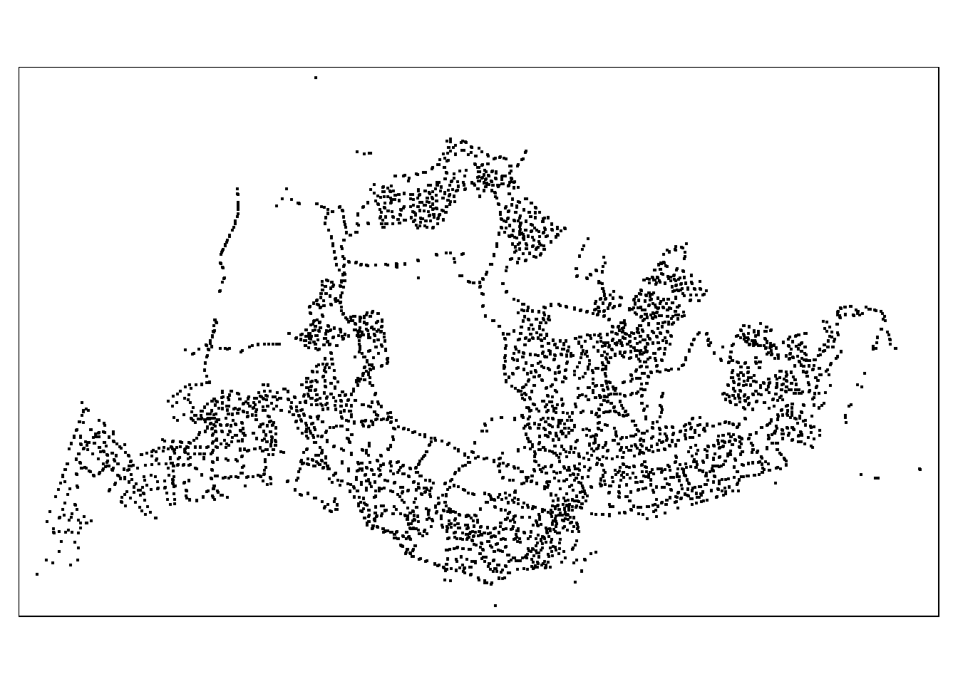
The st_crs() function is used to check for ESPG Code and Coordinate System of both geospatial files. In order to perform geoprocessing using different geospatial data sources, both need to be projected using similar coordinate systems and be assigned the correct EPSG code based on CRS.
st_crs(busstop)Coordinate Reference System:
User input: SVY21
wkt:
PROJCRS["SVY21",
BASEGEOGCRS["WGS 84",
DATUM["World Geodetic System 1984",
ELLIPSOID["WGS 84",6378137,298.257223563,
LENGTHUNIT["metre",1]],
ID["EPSG",6326]],
PRIMEM["Greenwich",0,
ANGLEUNIT["Degree",0.0174532925199433]]],
CONVERSION["unnamed",
METHOD["Transverse Mercator",
ID["EPSG",9807]],
PARAMETER["Latitude of natural origin",1.36666666666667,
ANGLEUNIT["Degree",0.0174532925199433],
ID["EPSG",8801]],
PARAMETER["Longitude of natural origin",103.833333333333,
ANGLEUNIT["Degree",0.0174532925199433],
ID["EPSG",8802]],
PARAMETER["Scale factor at natural origin",1,
SCALEUNIT["unity",1],
ID["EPSG",8805]],
PARAMETER["False easting",28001.642,
LENGTHUNIT["metre",1],
ID["EPSG",8806]],
PARAMETER["False northing",38744.572,
LENGTHUNIT["metre",1],
ID["EPSG",8807]]],
CS[Cartesian,2],
AXIS["(E)",east,
ORDER[1],
LENGTHUNIT["metre",1,
ID["EPSG",9001]]],
AXIS["(N)",north,
ORDER[2],
LENGTHUNIT["metre",1,
ID["EPSG",9001]]]]According to epsg.io, Singapore’s coordinate system is SVY21 with EPSG 3414
- busstop is projected in SVY21 with EPSG 9001 – this will require re-assignment of EPSG code to 3414
This is done using the st_set_crs() function
# Assign EPSG code
busstop <- st_set_crs(
busstop,
3414
) %>%
# rename bus stop origin for easy join to main dataframe
mutate(
ORIGIN_PT_CODE = as.factor(BUS_STOP_N)
) %>%
select(
ORIGIN_PT_CODE,
LOC_DESC,
geometry
) %>%
# change all column names to lowercase
rename_with(
tolower, everything()
)
# Confirm EPSG code
st_crs(busstop)Coordinate Reference System:
User input: EPSG:3414
wkt:
PROJCRS["SVY21 / Singapore TM",
BASEGEOGCRS["SVY21",
DATUM["SVY21",
ELLIPSOID["WGS 84",6378137,298.257223563,
LENGTHUNIT["metre",1]]],
PRIMEM["Greenwich",0,
ANGLEUNIT["degree",0.0174532925199433]],
ID["EPSG",4757]],
CONVERSION["Singapore Transverse Mercator",
METHOD["Transverse Mercator",
ID["EPSG",9807]],
PARAMETER["Latitude of natural origin",1.36666666666667,
ANGLEUNIT["degree",0.0174532925199433],
ID["EPSG",8801]],
PARAMETER["Longitude of natural origin",103.833333333333,
ANGLEUNIT["degree",0.0174532925199433],
ID["EPSG",8802]],
PARAMETER["Scale factor at natural origin",1,
SCALEUNIT["unity",1],
ID["EPSG",8805]],
PARAMETER["False easting",28001.642,
LENGTHUNIT["metre",1],
ID["EPSG",8806]],
PARAMETER["False northing",38744.572,
LENGTHUNIT["metre",1],
ID["EPSG",8807]]],
CS[Cartesian,2],
AXIS["northing (N)",north,
ORDER[1],
LENGTHUNIT["metre",1]],
AXIS["easting (E)",east,
ORDER[2],
LENGTHUNIT["metre",1]],
USAGE[
SCOPE["Cadastre, engineering survey, topographic mapping."],
AREA["Singapore - onshore and offshore."],
BBOX[1.13,103.59,1.47,104.07]],
ID["EPSG",3414]]busstop is now assigned the correct EPSG code.
4 Data Preparation
To narrow down the scope of the study, only patterns pertaining to peak hour trips will be analysed.
flowchart TD A[bus stops] -->|placed within| B[hexagon areas] -->|traffic| C(weekday morning) -.- G(6 - 9am) B -->|traffic| D(weekday afternoon) -.- H(5 - 8pm) B -->|traffic| E(weekend/PH morning) -.- I(11am - 2pm) B -->|traffic| F(weekend/PH evening) -.- J(4 - 7pm)
4.1 Aspatial Data Preparation
ORIGIN_PT_CODE and DESTINATION_PT_CODE are in character format. These represent the busstop locations, and are thus transformed into factors (categorical data type) for further analysis
busod <- busod %>%
mutate(
ORIGIN_PT_CODE = as.factor(ORIGIN_PT_CODE),
DESTINATION_PT_CODE = as.factor(DESTINATION_PT_CODE)
)The following code chunk involves multiple steps to prepare the relevant data needed for further analysis:
- Categorize trips by peak period based on day and time by creating a new categorical variable, period, and filtering the data using nested
ifelse()conditions filter()out non peak periods- Compute number of trips per origin busstop per month for each period using
group_by()andsummarise()
busod_agg <- busod %>%
# Categorize trips under period based on day and timeframe
mutate(period = ifelse(DAY_TYPE == "WEEKDAY" &
TIME_PER_HOUR >= 6 & TIME_PER_HOUR <= 9,
"Weekday morning peak",
ifelse(DAY_TYPE == "WEEKDAY" &
TIME_PER_HOUR >= 17 & TIME_PER_HOUR <= 20,
"Weekday evening peak",
ifelse(DAY_TYPE == "WEEKENDS/HOLIDAY" &
TIME_PER_HOUR >= 11 & TIME_PER_HOUR <= 14,
"Weekend/PH morning peak",
ifelse(DAY_TYPE == "WEEKENDS/HOLIDAY" &
TIME_PER_HOUR >= 16 & TIME_PER_HOUR <= 19,
"Weekend/PH evening peak",
"Others"))))
) %>%
# Only retain needed periods for analysis
filter(
period != "Others"
) %>%
# compute number of trips per origin busstop per month for each period
group_by(
YEAR_MONTH,
period,
ORIGIN_PT_CODE
) %>%
summarise(
num_trips = sum(TOTAL_TRIPS)
) %>%
# change all column names to lowercase
rename_with(
tolower, everything()
) %>%
ungroup()5 What is the Distribution of Passenger Traffic across peak periods?
It is important to understand the distribution of passenger trip volume across different time periods in a day for better urban traffic management and alleviating commuter congestion. Geospatial analysis methods enable us to visualise areas where commuter traffic is particularly dense, or uncover daily commuter patterns.
As a start, we will look at the distribution of passenger trips for different periods in August 2023:
code block
set_urbn_defaults(style = "print")
bus08_density <- busod_agg %>%
filter(
year_month == "2023-08"
) %>%
ggplot(
aes(x = num_trips,
y = period,
fill = period,
color = period)
) +
# create density ridgeplot to visualise distribution
geom_rain(
size = 3,
alpha = .7,
# Adding outline to boxplot
boxplot.args = list(
color = "grey20", outlier.shape = NA),
violin.args = list(alpha = .7)
) +
scale_x_continuous(
labels = scales::number_format(accuracy = 1),
breaks = scales::pretty_breaks(n = 5)
) +
labs(
title = "Aug 2023: Higher Passenger Traffic recorded on Weekday Peak Periods",
subtitle = "Wider range of trips recorded during weekdays, suggestive of possible congestion"
) +
theme(
axis.title.y = element_blank(),
axis.title.x = element_blank(),
axis.ticks.y = element_blank(),
legend.position = "none" # Remove the legend
)
bus08_density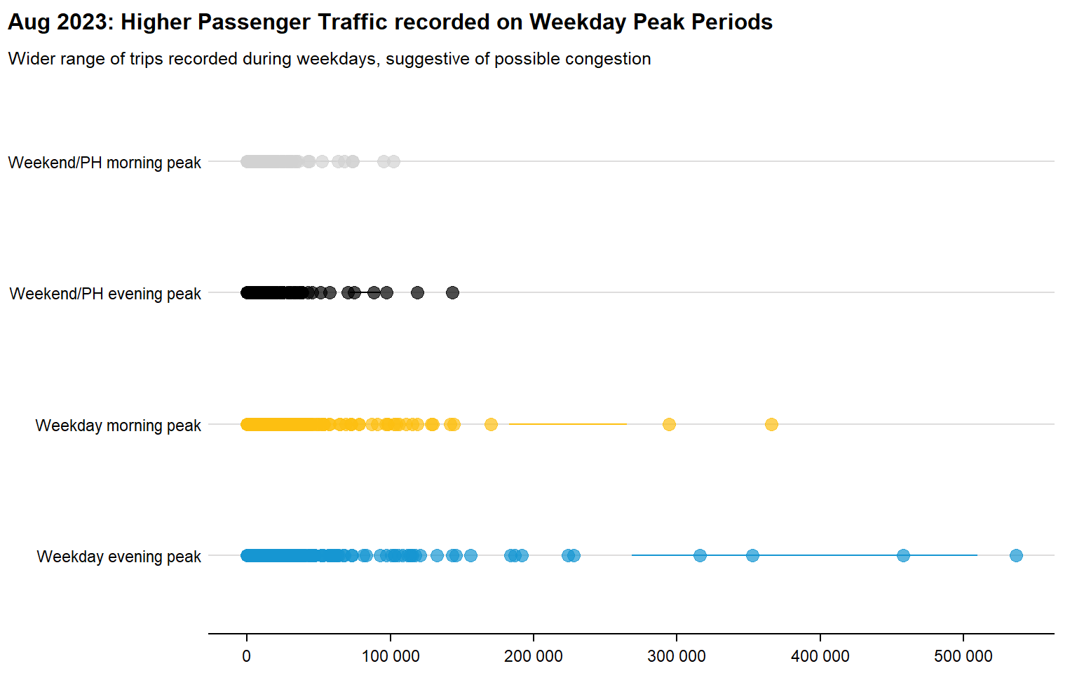
Initial Insights
- The range of passenger volume is much larger during weekday peak hours compared to weekends/public holidays
- All four peak periods show a right-skewed distribution, with several outliers recording a much higher passenger volume
- This could be suggestive of high traffic in busy locations. especially in the CBD area or Bus/MRT interchanges
- Further analysis could be done to determine if they are in similar areas, to determine potential hot spots
5.1 Does this distribution change over time?
To understand if this distribution is unique to the month of August, or records similar trends throughout the months, the distribution of passenger traffic across peak periods over 3 months is compared:
code block
bus_density <- busod_agg %>%
ggplot(
aes(x = period,
y = num_trips,
fill = period,
color = period)
) +
geom_violin(
position = position_nudge(x = .2, y = 0), alpha = .8
) +
geom_point(
aes(y = num_trips,
color = period),
position = position_jitter(width = .15),
size = .5,
alpha = 0.8
) +
geom_boxplot(
width = .1,
outlier.shape = NA,
alpha = 0.5
) +
facet_wrap(~year_month,
nrow = 1
) +
scale_y_continuous(
labels = scales::number_format(accuracy = 1),
breaks = scales::pretty_breaks(n = 3)
) +
labs(
title = "Aug - Oct 2023: Similar distributions of Passenger Traffic"
) +
theme(
axis.title.y = element_blank(),
axis.title.x = element_blank(),
axis.ticks.y = element_blank(),
axis.ticks.x = element_blank(),
legend.position = "none"
) +
coord_flip()
bus_density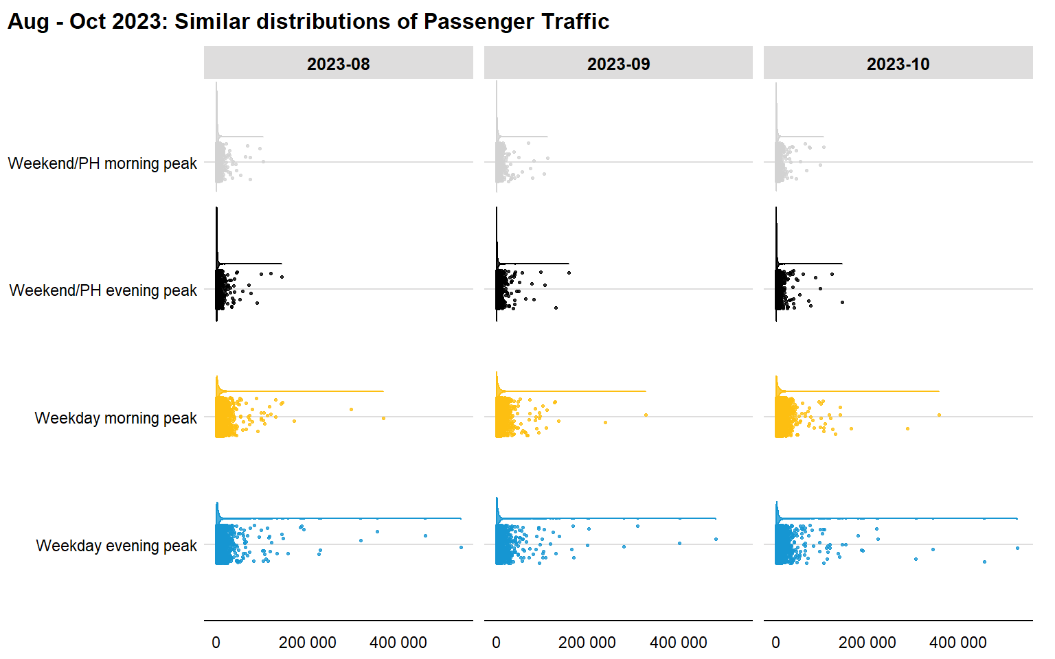
The density plots above reveal that the distribution of number of trips recorded over a 3-month period are very similar. It is thus reasonable to deduce that there are several bus stops with very high passenger volume, especially on weekday evening peak periods – if these bus stops are within close proximity to each other, it could point towards possible hot spots for traffic congestion.
As the trend does not change significantly over the months, further geospatial analysis is conducted on August 2023 passenger traffic data to locate these potential hot spots.
5.2 Extracting Specific data for study
August 2023 Passenger volume data is filtered out using the following code, and a pivot table is created such that each row represents a single bus stop:
# Extract august data and store as separate dataframe
busod_08 <- busod_agg %>%
filter(
year_month == "2023-08"
) %>%
# get each row as a bus stop code with peak period trips as columns
pivot_wider(
names_from = period,
values_from = num_trips
) %>%
select(2:6)
DT::datatable(busod_08,
options = list(pageLength = 8),
rownames = FALSE)5.3 Creating Spatial Polygon Dataframe
Using left_join to map busstops by bus stop code
busod_08_sf <- left_join(busstop, busod_08, by = "origin_pt_code")
busod_08_sfSimple feature collection with 5161 features and 6 fields
Geometry type: POINT
Dimension: XY
Bounding box: xmin: 3970.122 ymin: 26482.1 xmax: 48284.56 ymax: 52983.82
Projected CRS: SVY21 / Singapore TM
First 10 features:
origin_pt_code loc_desc Weekday evening peak
1 22069 OPP CEVA LOGISTICS 43
2 32071 AFT TRACK 13 NA
3 44331 BLK 239 1742
4 96081 GRACE INDEPENDENT CH 399
5 11561 BLK 166 195
6 66191 AFT CORFE PL 362
7 23389 PEC LTD 406
8 54411 BLK 527 1314
9 28531 BLK 536 3789
10 96139 BLK 148 1420
Weekday morning peak Weekend/PH evening peak Weekend/PH morning peak
1 15 12 6
2 NA 1 NA
3 2124 546 700
4 307 84 110
5 190 61 81
6 399 173 158
7 35 84 10
8 3112 497 1436
9 9258 1873 1970
10 5030 710 858
geometry
1 POINT (13576.31 32883.65)
2 POINT (13228.59 44206.38)
3 POINT (21045.1 40242.08)
4 POINT (41603.76 35413.11)
5 POINT (24568.74 30391.85)
6 POINT (30951.58 38079.61)
7 POINT (12476.9 32211.6)
8 POINT (30329.45 39373.92)
9 POINT (14993.31 36905.61)
10 POINT (41642.81 36513.9)busod_08_sf is a spatial point dataframe. This is not particularly useful when dealing with spatial autocorrelation analysis, as ‘areas’ need to be defined as planes in space (polygons instead of points). The following code chunks place these bus stops into a hexagon grid:
Step 1: Create a hexagon grid frame
- Use the
st_make_grid()function cellsizeargument units are the same as the dataframe’s. As busod_08_sf is projected in ESPG code 3414, the unit is in meters and defines the width of the hexagon. This is set to 500m.- Assign a
hex_idto each hexagon as primary key
output: Spatial polygons, with hex_id and geometry data
busod_08_hex <- st_make_grid(
busod_08_sf,
cellsize = 500,
square = FALSE
) %>%
st_sf() %>%
rowid_to_column("hex_id")Step 2: Create Attribute dataframe using hex id instead of busstop code
As each hexagon area may contain more than a single bus stop, we need to use hex_id as primary key. The following steps are taken to group the attributes by hex_id:
- Use the
st_join()function withjoin = st_withinto place busstop points within the hexagon areas st_set_grometry(NULL)argument removes the geospatial layergroup_by()to get uniquehex_idper rowsummarise()to compute the aggregate number of bus stops and trips per peak period for each hexagon areareplace(is.na(.), 0)replaces allNAvalues with 0
output: Aspatial Attributes dataframe, with hex_id as primary key
busod_08_stops <- st_join(
busod_08_sf,
busod_08_hex,
join = st_within
) %>%
st_set_geometry(NULL) %>%
group_by(
hex_id
) %>%
summarise(
n_busstops = n(),
busstop_codes = str_c(origin_pt_code, collapse = ","),
`Weekday morning peak` = sum(`Weekday morning peak`),
`Weekday evening peak` = sum(`Weekday evening peak`),
`Weekend/PH morning peak` = sum(`Weekend/PH morning peak`),
`Weekend/PH evening peak` = sum(`Weekend/PH evening peak`)
) %>%
replace(is.na(.), 0) %>%
ungroup()Step 3: Create Spatial Polygon dataframe by joining
left_jointhe new busod_08_stops aspatial dataframe to busod_08_hex hexagon geospatial layer byhex_idto add attributes to the spatial polygon dataframefilterout the hexagons with no bus stops
Output: Spatial Polygon Dataframe
busod_08_hex <- busod_08_hex %>%
left_join(busod_08_stops,
by = "hex_id"
) %>%
replace(is.na(.), 0)
bustraffic08 <- filter(busod_08_hex,
n_busstops > 0)The following map shows each area coloured by bus stop density:
code block
tmap_mode("view")
bustraffic08_map <- tm_basemap("CartoDB.Positron") +
tm_shape(bustraffic08) +
tm_fill(
col = "n_busstops",
palette = "PuBu",
style = "cont",
id = "hex_id",
popup.vars = c("No. of bus stops: " = "n_busstops",
"Bus Stop codes: " = "busstop_codes"),
title = " "
) +
tm_layout(
# Set legend.show to FALSE to hide the legend
legend.show = FALSE
)
bustraffic08_map6 Does an area with higher bus stop density record higher passenger volume?
code block
weekday_m_scat <- ggplot(
bustraffic08,
aes(x = as.factor(n_busstops),
y = `Weekday morning peak`,)
) +
geom_point(
alpha = .7
) +
ylim(0, 500000) +
scale_y_continuous(
breaks = scales::pretty_breaks(n = 6)
) +
labs(
title = "Weekday Morning Peak",
x = "No. Bus stops",
y = ""
) +
theme(
panel.grid = element_blank()
)
weekday_e_scat <- ggplot(
bustraffic08,
aes(x = as.factor(n_busstops),
y = `Weekday evening peak`,)
) +
geom_point(
alpha = .7
) +
ylim(0, 500000) +
labs(
title = "Weekday Evening Peak",
x = "No. Bus stops",
y = ""
) +
theme(
panel.grid = element_blank(),
axis.text.y = element_blank()
)
ph_m_scat <- ggplot(
bustraffic08,
aes(x = as.factor(n_busstops),
y = `Weekend/PH morning peak`,)
) +
geom_point(
alpha = .7,
color = "salmon"
) +
ylim(0, 500000) +
scale_y_continuous(
labels = scales::number_format(accuracy = 1),
breaks = scales::pretty_breaks(n = 6)
) +
labs(
title = "Weekend/PH Morning Peak",
x = "No. Bus stops",
y = ""
) +
theme(
panel.grid = element_blank()
)
ph_e_scat <- ggplot(
bustraffic08,
aes(x = as.factor(n_busstops),
y = `Weekend/PH evening peak`,)
) +
geom_point(
alpha = .7,
color = "salmon"
) +
ylim(0, 500000) +
labs(
title = "Weekend/PH Evening Peak",
x = "No. Bus stops",
y = ""
) +
theme(
panel.grid = element_blank(),
axis.text.y = element_blank()
)
weekday_patch <- (weekday_m_scat + weekday_e_scat)
weekend_patch <- (ph_m_scat + ph_e_scat)
fullpatch <- (weekday_patch / weekend_patch) +
plot_annotation(title = "Areas with highest bus stop density not the most congested")
fullpatch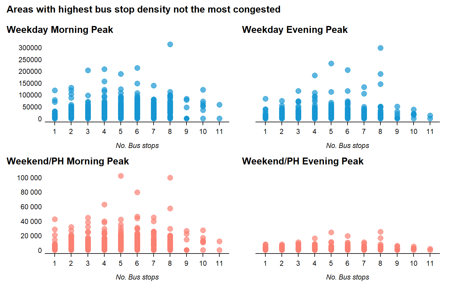
- Passenger trip volume seems to he highest in areas with 5 - 8 number of bus stops
- Areas with the highest bus stop density (9 - 11) Did not record the highest passenger traffic across all peak periods
- This suggests that there may be an optimum number of bus stops per 500m width area that would reduce congestion
7 Where are the passenger volume hotspots on weekday peak periods??
Based on the following animated map, there are several areas that record similarly high passenger traffic during morning and evening peak period:
code block
weekday_hourly <- busod %>%
filter(YEAR_MONTH == "2023-08") %>%
filter(DAY_TYPE == "WEEKDAY") %>%
group_by(
ORIGIN_PT_CODE,
TIME_PER_HOUR
) %>%
summarise(
TOTAL_TRIPS = sum(TOTAL_TRIPS)
) %>%
rename_with(
tolower, everything()
) %>%
ungroup()
wd_hourly_sf <- left_join(busstop, weekday_hourly, by = "origin_pt_code")
wd_hourly_hex <- st_make_grid(
wd_hourly_sf,
cellsize = 500,
square = FALSE
) %>%
st_sf() %>%
rowid_to_column("hex_id")
wd_hourly_stops <- st_join(
wd_hourly_sf,
wd_hourly_hex,
join = st_within
) %>%
st_set_geometry(NULL) %>%
group_by(
hex_id,
time_per_hour
) %>%
summarise(
n_busstops = n(),
busstop_codes = str_c(origin_pt_code, collapse = ","),
total_trips = sum(total_trips)
) %>%
replace(is.na(.), 0) %>%
ungroup()
wd_hourly_hex <- wd_hourly_hex %>%
left_join(wd_hourly_stops,
by = "hex_id"
) %>%
replace(is.na(.), 0)
wd_hourly08 <- filter(wd_hourly_hex,
n_busstops > 0)
wd_hourly_map <- tm_shape(wd_hourly08) +
tm_fill(
col = "total_trips",
palette = "OrRd",
style = "cont"
) +
tm_layout(
title = "Weekday Passenger Volume",
frame = FALSE
) +
tm_facets(
along = "time_per_hour",
free.coords = FALSE
)
# Save animation as gif
tmap_animation(wd_hourly_map,
"wd_hourly_map.gif",
loop = TRUE,
delay = 40,
outer.margins = NA,)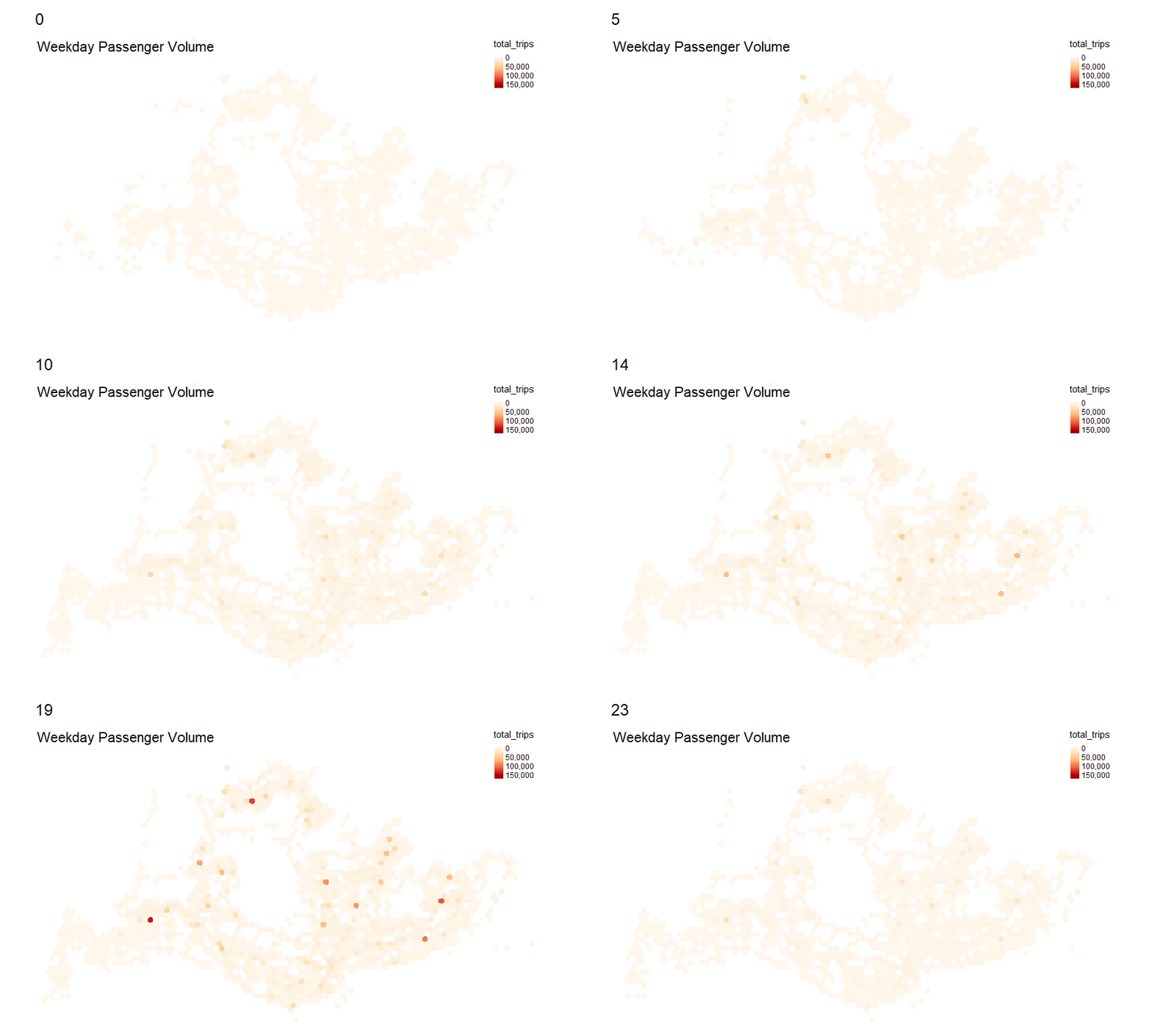
The following maps compare the passenger traffic distribution between weekday morning and evening peak periods:
7.1 Continuous Intervals
style = "cont" argument is specified to fill the hexagons along a continuous colour scale according to passenger trip volume.
code block
bus08_facet <- tm_shape(bustraffic08) +
tm_fill(c("Weekday morning peak", "Weekday evening peak"),
palette = "Reds",
style = "cont",
alpha = .7,
popup.vars = c("No. of bus stops: " = "n_busstops",
"Weekday Morning traffic: " = "Weekday morning peak",
"Weekday Evening traffic: " = "Weekday evening peak",
"Bus Stop codes: " = "busstop_codes")
) +
tm_scale_bar(width = 0.15) +
tm_layout(
title = c("Weekday morning peak", "Weekday evening peak"),
panel.labels = c("Weekday morning peak", "Weekday evening peak")
) +
tm_facets(
sync = TRUE,
ncol = 1
)
bus08_facet7.2 Binned by Quantiles
style = "quantile" argument is used categorically bin the variable based on quantile values. The traffic appears far more congested using this binning method compared to the continuous scale, and is largely due to the highly skewed distribution of the variable. It is thus not a conclusive way of determining which areas are true hot spots based on volume of trips.
code block
bus08_facet2 <- tm_shape(bustraffic08) +
tm_fill(c("Weekday morning peak", "Weekday evening peak"),
palette = "Reds",
style = "quantile",
alpha = .7,
popup.vars = c("No. of bus stops: " = "n_busstops",
"Weekday Morning traffic: " = "Weekday morning peak",
"Weekday Evening traffic: " = "Weekday evening peak",
"Bus Stop codes: " = "busstop_codes")
) +
tm_scale_bar(width = 0.15) +
tm_layout(
title = c("Weekday morning peak", "Weekday evening peak"),
panel.labels = c("Weekday morning peak", "Weekday evening peak")
) +
tm_facets(
sync = TRUE,
ncol = 1
)
bus08_facet27.3 Binned by jenks algorithm
style = "jenks" argument is used to ‘cluster’ groups with similar values and maximize the difference between each group. It is based on the Jenks natural breaks classification method, a data clustering algorithm used to determine the best arrangement of values and assign them into ‘classes’. This is chosen over equal or quantile binning due to the wide range of values present in the distribution.
code block
bus08_facet3 <- tm_shape(bustraffic08) +
tm_fill(c("Weekday morning peak", "Weekday evening peak"),
palette = "Reds",
style = "jenks",
alpha = .7,
popup.vars = c("No. of bus stops: " = "n_busstops",
"Weekday Morning traffic: " = "Weekday morning peak",
"Weekday Evening traffic: " = "Weekday evening peak",
"Bus Stop codes: " = "busstop_codes")
) +
tm_scale_bar(width = 0.15) +
tm_layout(
title = c("Weekday morning peak", "Weekday evening peak"),
panel.labels = c("Weekday morning peak", "Weekday evening peak")
) +
tm_facets(
sync = TRUE,
ncol = 1
)
bus08_facet3.
While the continuous colour-scale map showed more isolated pockets of areas as potential hotspots, the quantile binning and jenks algorithm revealed a more clustered distribution of hotspot areas.
Comparing the maps, several Areas have been identified as Weekday Peak high passenger volume hotspots. These are mostly areas encompassing an MRT Station and/or Bus Interchange, and are listed out by hexagon ID below:
hex_2411 <- busstop %>%
filter(
origin_pt_code %in% c("46649","46339","46009","46321","46641","46639","46631","46329")
) %>%
st_set_geometry(NULL) %>%
select(
origin_pt_code, loc_desc
)
DT::datatable(hex_2411)hex_3239 <- busstop %>%
filter(
origin_pt_code %in% c("54247","54339","54391","54261","54009","54399")
) %>%
st_set_geometry(NULL) %>%
select(
origin_pt_code, loc_desc
)
DT::datatable(hex_3239)hex_4349 <- busstop %>%
filter(
origin_pt_code %in% c("84031","84139","84131","84009","84039")
) %>%
st_set_geometry(NULL) %>%
select(
origin_pt_code, loc_desc
)
DT::datatable(hex_4349)hex_4018 <- busstop %>%
filter(
origin_pt_code %in% c("65079","65191","65199","65071")
) %>%
st_set_geometry(NULL) %>%
select(
origin_pt_code, loc_desc
)
DT::datatable(hex_4018)hex_2054 <- busstop %>%
filter(
origin_pt_code %in% c("20019","17179","17171")
) %>%
st_set_geometry(NULL) %>%
select(
origin_pt_code, loc_desc
)
DT::datatable(hex_2054)8 Are these the same hotspots as Weekend/Public Holiday peak periods??
The following maps compare the passenger traffic distribution between weekend/Public holiday morning and evening peak periods:
8.1 Continuous Intervals
code block
ph_bus08_facet <- tm_shape(bustraffic08) +
tm_fill(c("Weekend/PH morning peak", "Weekend/PH evening peak"),
palette = "Purples",
style = "cont",
alpha = .7,
popup.vars = c("No. of bus stops: " = "n_busstops",
"Weekend/PH Morning traffic: " = "Weekday morning peak",
"Weekend/PH Evening traffic: " = "Weekday evening peak",
"Bus Stop codes: " = "busstop_codes")
) +
tm_scale_bar(width = 0.15) +
tm_layout(
title = c("Weekend/PH morning peak", "Weekend/PH evening peak")
) +
tm_facets(
sync = TRUE,
ncol = 1
)
ph_bus08_facet8.2 Binned by quantile
code block
tmap_mode("view")
ph_bus08_facet2 <- tm_shape(bustraffic08) +
tm_fill(c("Weekend/PH morning peak", "Weekend/PH evening peak"),
palette = "Purples",
style = "quantile",
alpha = .7,
popup.vars = c("No. of bus stops: " = "n_busstops",
"Weekend/PH Morning traffic: " = "Weekday morning peak",
"Weekend/PH Evening traffic: " = "Weekday evening peak",
"Bus Stop codes: " = "busstop_codes")
) +
tm_scale_bar(width = 0.15) +
tm_layout(
title = c("Weekend/PH morning peak", "Weekend/PH evening peak")
) +
tm_facets(
sync = TRUE,
ncol = 1
)
ph_bus08_facet28.3 Binned by jenks algorithm
code block
ph_bus08_facet3 <- tm_shape(bustraffic08) +
tm_fill(c("Weekend/PH morning peak", "Weekend/PH evening peak"),
palette = "Purples",
style = "jenks",
alpha = .7,
popup.vars = c("No. of bus stops: " = "n_busstops",
"Weekend/PH Morning traffic: " = "Weekday morning peak",
"Weekend/PH Evening traffic: " = "Weekday evening peak",
"Bus Stop codes: " = "busstop_codes")
) +
tm_scale_bar(width = 0.15) +
tm_layout(
title = c("Weekend/PH morning peak", "Weekend/PH evening peak")
) +
tm_facets(
sync = TRUE,
ncol = 1
)
ph_bus08_facet3The ‘clustered’ maps above reveal denser hotspots in the north and central regions compared to Weekday peak periods. However, similarly high passenger traffic was recording in specific areas, identified and listed below:
hex_3292 <- busstop %>%
filter(
origin_pt_code %in% c("01013","01119","01112","01019","01012","04029","07569","07561")
) %>%
st_set_geometry(NULL) %>%
select(
origin_pt_code, loc_desc
)
DT::datatable(hex_3292)hex_3014 <- busstop %>%
filter(
origin_pt_code %in% c("09011","09022","09048","09047","09023")
) %>%
st_set_geometry(NULL) %>%
select(
origin_pt_code, loc_desc
)
DT::datatable(hex_3014)hex_2135 <- busstop %>%
filter(
origin_pt_code %in% c("46211","46219")
) %>%
st_set_geometry(NULL) %>%
select(
origin_pt_code, loc_desc
)
DT::datatable(hex_2135)Weekday vs Weekend/PH Peak Periods
- Key hotspot areas were similar, especially in larger heartland areas with busy MRT stations and bus interchanges
- Jenks algorithm revealed smaller ‘clusters’ of hot spots during weekend peak periods compared to weekday peak periods, although both day types had similar highest passenger traffic areas
- The visualised distribution of passenger volume using continuous scale versus binned intervals reveals different patterns, and further investigation needs to be conducted to determine if those areas are truly spatially clustered or are outliers in the overall distribution
9 Which areas are likely to have passenger congestion?
To uncover any trends in spatial clustering, we conduct the local Moran’s I Test to determine if there are clusters of high traffic, or if there are areas that are outliers in the overall spatial distribution.
Computing this LISA statistic for each observation gives an indication of the extent of significant spatial clustering of similar values around that observation and helps in determining areas that are passenger traffic-heavy during the peak hour periods.
9.1 Computing local Moran’s I statistics
The code chunk below performs the following actions:
mutatecreates 2 new columns, nb and wt- nb stores the Queen’c contiguity weight matrix, computed using
st_contiguity - wt stores the row-standardised weight matrix
wm08 <- busod_08_hex %>%
mutate(nb = st_contiguity(geometry),
wt = st_weights(nb,
style = "W"),
.before = 1)The following code runs a Monte Carlo simulation of Local Moran’s I on weekday morning peak traffic.This function returns the following values as separate columns:
- ii (Moran’s I for each observation): the local spatial autocorrelation for each hexagon. +ve values suggest clustering while -ve values suggest dispersion.
- E_ii (Expected Moran’s I for each observation): the expected value of Moran’s I under spatial randomness, based on the assumption that there is no spatial autocorrelation.
- var_ii (Variance of Ii): the variability of the Moran’s I values across observations
- z_ii (Z-score): A standardized score that measures how many standard deviations an observed Moran’s I deviates from the expected Moran’s I. +ve scores indicate higher correlation than expected
- p_ii (p-value): the probability of observing the given Moran’s I under the assumption of spatial randomness. A p-value less than the chosen significance level (e.g., 0.05) suggests that the spatial pattern is statistically significant.
- p_ii_sim (simulated p-value): the p-value based on monte carlo simulation of 1000 trials
- mean, median, pysal: the cluster category based spatial patterns
# set seed to ensure that results from simulation are reproducible
set.seed(8888)
# Weekday morning
lisa08_wdm <- wm08 %>%
mutate(local_moran = local_moran(`Weekday morning peak`,
nb,
wt,
nsim = 999),
.before = 1) %>%
unnest(local_moran) %>%
# only retain hexagons with a bus stop
filter(n_busstops > 0)
# Weekday evening
lisa08_wde <- wm08 %>%
mutate(local_moran = local_moran(`Weekday evening peak`,
nb,
wt,
nsim = 999),
.before = 1) %>%
unnest(local_moran) %>%
# only retain hexagons with a bus stop
filter(n_busstops > 0)9.2 Step 3: Visualise I statistic and p-value
An area could be identified as a cluster or an outlier based on I statistic value and p-value:
- outlier: significant and negative i value (area is associated with relatively low i values of neighbors)
- cluster: significant and positive i value (area is associated with relatively high i values of neighbors)
code block
# Set map to static
tmap_mode("plot")
# weekday morning moran I values
map_wdm_moran08 <- tm_shape(lisa08_wdm) +
tm_fill(
col = "ii",
palette = "OrRd",
style = "pretty",
title = "Local Moran's I"
) +
tm_layout(main.title = "Weekday Morning Peak Traffic",
main.title.size = 1,
main.title.position = "center",
legend.position = c("left", "top"),
legend.height = .6,
legend.width = .2,
frame = FALSE
)
# weekday morning p-values
map_wdm_pvalue <- tm_shape(lisa08_wdm) +
tm_fill(
col = "p_ii_sim",
palette = "-BuGn",
alpha = .8,
breaks = c(0, 0.001, 0.01, 0.05, 1),
labels = c("0.001", "0.01", "0.05", "Not Sig"),
title = "p-value"
) +
tm_layout(main.title = "p-values of Local Moran's I",
main.title.size = 0.8,
main.title.position = "center",
legend.position = c("right", "top"),
legend.height = .5,
legend.width = .2,
frame = FALSE
)
# weekday evening moran I values
map_wde_moran08 <- tm_shape(lisa08_wde) +
tm_fill(
col = "ii",
palette = "OrRd",
style = "pretty",
title = "Local Moran's I"
) +
tm_layout(main.title = "Weekday Evening Peak Traffic",
main.title.size = 1,
main.title.position = "center",
legend.position = c("left", "top"),
legend.height = .6,
legend.width = .2,
frame = FALSE
)
# weekday evening p-values
map_wde_pvalue <- tm_shape(lisa08_wde) +
tm_fill(
col = "p_ii_sim",
palette = "-BuGn",
alpha = .8,
breaks = c(0, 0.001, 0.01, 0.05, 1),
labels = c("0.001", "0.01", "0.05", "Not Sig"),
title = "p-value"
) +
tm_layout(main.title = "p-values of Local Moran's I",
main.title.size = 0.8,
main.title.position = "center",
legend.position = c("right", "top"),
legend.height = .5,
legend.width = .2,
frame = FALSE
)
tmap_arrange(map_wdm_moran08, map_wdm_pvalue,
map_wde_moran08, map_wde_pvalue,
ncol = 2)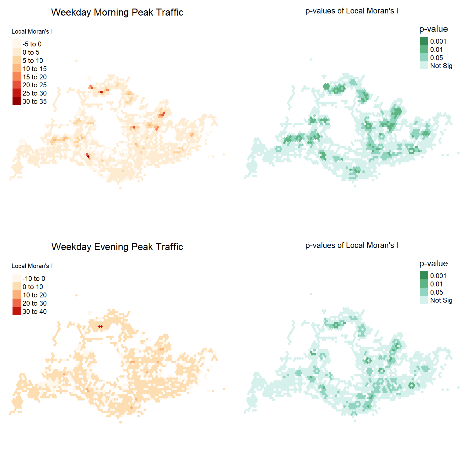
code block
set.seed(8888)
# Compute local moran's I simulation for weekend/PH morning peak
lisa08_phm <- wm08 %>%
mutate(local_moran = local_moran(`Weekend/PH morning peak`,
nb,
wt,
nsim = 999),
.before = 1) %>%
unnest(local_moran) %>%
# only retain hexagons with a bus stop
filter(n_busstops > 0)
# Compute local moran's I simulation for weekend/PH evening peak
lisa08_phe <- wm08 %>%
mutate(local_moran = local_moran(`Weekend/PH evening peak`,
nb,
wt,
nsim = 999),
.before = 1) %>%
unnest(local_moran) %>%
# only retain hexagons with a bus stop
filter(n_busstops > 0)code block
# Set map to static
tmap_mode("plot")
# weekend/PH moran I values
map_phm_moran08 <- tm_shape(lisa08_phm) +
tm_fill(
col = "ii",
palette = "RdPu",
style = "pretty",
title = "Local Moran's I"
) +
tm_layout(main.title = "Weekend/PH Morning Peak Traffic",
main.title.size = 1,
main.title.position = "center",
legend.position = c("left", "top"),
legend.height = .6,
legend.width = .2,
frame = FALSE
)
# weekend/PH p-values
map_phm_pvalue <- tm_shape(lisa08_phm) +
tm_fill(
col = "p_ii_sim",
palette = "-BuGn",
alpha = .8,
breaks = c(0, 0.001, 0.01, 0.05, 1),
labels = c("0.001", "0.01", "0.05", "Not Sig"),
title = "p-value"
) +
tm_layout(main.title = "p-values of Local Moran's I",
main.title.size = 0.8,
main.title.position = "center",
legend.position = c("right", "top"),
legend.height = .5,
legend.width = .2,
frame = FALSE
)
# weekend/PH moran I values
map_phe_moran08 <- tm_shape(lisa08_phe) +
tm_fill(
col = "ii",
palette = "RdPu",
style = "pretty",
title = "Local Moran's I"
) +
tm_layout(main.title = "Weekend/PHEvening Peak Traffic",
main.title.size = 1,
main.title.position = "center",
legend.position = c("left", "top"),
legend.height = .6,
legend.width = .2,
frame = FALSE
)
# weekend/PH evening p-values
map_phe_pvalue <- tm_shape(lisa08_phe) +
tm_fill(
col = "p_ii_sim",
palette = "-BuGn",
alpha = .8,
breaks = c(0, 0.001, 0.01, 0.05, 1),
labels = c("0.001", "0.01", "0.05", "Not Sig"),
title = "p-value"
) +
tm_layout(main.title = "p-values of Local Moran's I",
main.title.size = 0.8,
main.title.position = "center",
legend.position = c("right", "top"),
legend.height = .5,
legend.width = .2,
frame = FALSE
)
tmap_arrange(map_phm_moran08, map_phm_pvalue,
map_phe_moran08, map_phe_pvalue,
ncol = 2)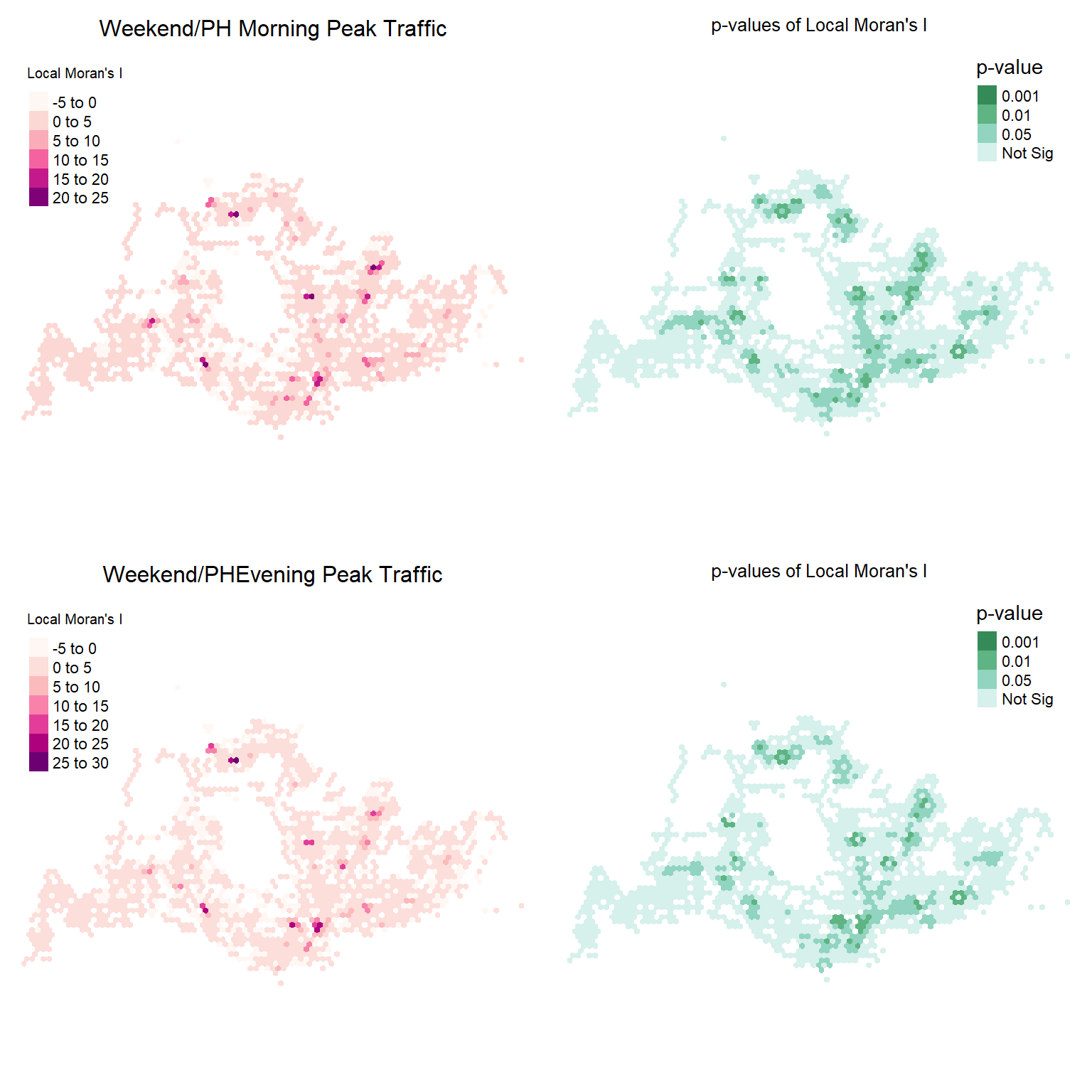
From comparing the maps above, we can detect multiple clusters that are significant and possess high, positive Local Moran’s I values. In general, there are more clusters during Weekday morning peak hours compared to evening, while the number of clusters during Weekends or Public holiday morning and evening peak periods do not show large variation. To visualise the extent of the spatial clustering, we look at the mean Local Moran’s I cluster quadrants, computed as variable mean.
9.3 Visualising Local Moran Clusters
The spatial clusters are visualised in the map below, with one showing all values and the other displaying only statistically significant clusters (p-value <0.05):
code block
colors <- c("#4d5887", "#B1EDE8", "#f5bc5f", "salmon")
tmap_mode("plot")
mean_wdm <- lisa08_wdm %>%
filter(p_ii_sim < 0.05)
# All significant values
plot_wdm_all <-
tm_shape(lisa08_wdm) +
tm_fill(
col = "mean",
style = "cat",
palette = colors
) +
tm_layout(
main.title = "Local Moran Clusters (All)",
main.title.size = .8,
main.title.position = "center",
frame = FALSE)
plot_wdm_mean <-
tm_shape(lisa08_wdm) +
tm_polygons(
col = "#ffffff"
) +
tm_borders(col = NA) +
tm_shape(mean_wdm) +
tm_fill(
col = "mean",
style = "cat",
palette = colors
) +
tm_layout(
main.title = "Local Moran Clusters (Significant)",
main.title.size = .8,
main.title.position = "center",
frame = FALSE)
tmap_arrange(plot_wdm_all, plot_wdm_mean,
ncol = 2)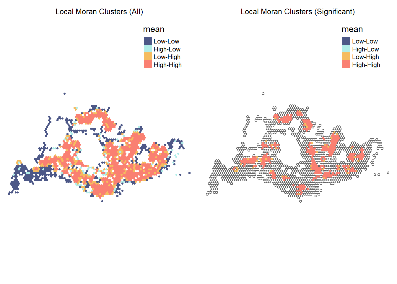
We can deduce that there are 2 main types of statistically significant clusters present during Weekday Morning Peak Periods:
- High-High clusters suggest spatial autocorrelation, indicating that areas with similar attribute values are clustered together to form possible hot spots for passenger congestion
- Low-High clusters suggest spatial outliers, where areas with dissimilar attribute values are located near each other. Passenger volume is much lower and these ares are not flagged for possible congestion.
9.4 Weekday Morning Peak Periods
code block
tmap_mode("view")
plot_wdm <- tm_basemap("CartoDB.Positron") +
tm_shape(mean_wdm) +
tm_fill(
c("Weekday morning peak", "mean"),
alpha = .7,
title = c("Passenger Volume", "Cluster"),
popup.vars = c("Hex ID: " = "hex_id",
"Cluster" = "mean",
"No. of bus stops: " = "n_busstops",
"Weekday Morning traffic: " = "Weekday morning peak",
"Bus Stop codes: " = "busstop_codes")
) +
tm_facets(
sync = TRUE,
ncol = 1
) +
tm_layout(
title = "Weekday Morning Peak Traffic",
title.size = 1
)
plot_wdm9.5 Weekday Evening Peak Periods
code block
mean_wde <- lisa08_wde %>%
filter(p_ii_sim < 0.05)
plot_wde <- tm_basemap("CartoDB.DarkMatter") +
tm_shape(mean_wde) +
tm_fill(
c("Weekday evening peak", "mean"),
alpha = .7,
title = c("Passenger Volume", "Cluster"),
popup.vars = c("Hex ID: " = "hex_id",
"Cluster" = "mean",
"No. of bus stops: " = "n_busstops",
"Weekday Morning traffic: " = "Weekday morning peak",
"Bus Stop codes: " = "busstop_codes")
) +
tm_facets(
sync = TRUE,
ncol = 1
) +
tm_layout(
title = "Weekday Evening Peak Traffic",
title.size = 1
)
plot_wde9.6 Weekend/Public Holiday Morning Peak Periods
code block
mean_phm <- lisa08_phm %>%
filter(p_ii_sim < 0.05)
tmap_mode("view")
plot_phm <- tm_basemap("CartoDB.Positron") +
tm_shape(mean_phm) +
tm_fill(
c("Weekend/PH morning peak", "mean"),
alpha = .7,
title = c("Passenger Volume", "Cluster"),
popup.vars = c("Hex ID: " = "hex_id",
"Cluster" = "mean",
"No. of bus stops: " = "n_busstops",
"Weekday Morning traffic: " = "Weekday morning peak",
"Bus Stop codes: " = "busstop_codes")
) +
tm_facets(
sync = TRUE,
ncol = 1
) +
tm_layout(
title = "Weekend/PH Morning Peak Traffic",
title.size = 1
)
plot_phm9.7 Weekend/Public Holiday Evening Peak Periods
code block
mean_phe <- lisa08_phe %>%
filter(p_ii_sim < 0.05)
tmap_mode("view")
plot_phe <- tm_basemap("CartoDB.DarkMatter") +
tm_shape(mean_phe) +
tm_fill(
c("Weekend/PH evening peak", "mean"),
alpha = .7,
title = c("Passenger Volume", "Cluster"),
popup.vars = c("Hex ID: " = "hex_id",
"Cluster" = "mean",
"No. of bus stops: " = "n_busstops",
"Weekday Morning traffic: " = "Weekday morning peak",
"Bus Stop codes: " = "busstop_codes")
) +
tm_facets(
sync = TRUE,
ncol = 1
) +
tm_layout(
title = "Weekend/PH Evening Peak Traffic",
title.size = 1
)
plot_pheThere are several key insights to be drawn from the maps presented above:
- Weekday Morning and Evening Peak Timings have similar hot spot clusters, concentrated around MRT Stations of residential neighbourhoods such as Woodlands, Yishun, Ang Mo Kio, etc.
- However, Weekday Evening Peak Periods reveal clusters of high traffic in the Central, CBD area as well. As the aggregation of trips is based on point of origin, this shows that the general traffic flows outward from the CBD area after working hours.
- Weekend/Public Holiday Morning and Evening Peak traffic have similar high-high clusters as well, even though the absolute volume of passenger trips is lower. This could be due to more people driving rather than commuting via bus.
- Hot spot clusters around residential neighborhoods’ MRT stations persists on Weekends/PH as well, suggesting a high population density in those areas.
10 Conclusion & Areas for further study
The insights presented above reveal traffic patterns that could be helpful for urban transport management. In particular, it shows areas of high passenger traffic, that could be alleviated by increasing bus frequency. However, more information is needed to optimize this:
As the study considers only origin bus stop to compute passenger volume, it does not accurately capture the flow of the passenger journey and where the passengers alight. This data could help with understanding denser or more popular areas amongst bus users.
The study does not provide data on bus number or bus route. Having this information could help in investigating the more popular bus routes as well as cross reference this with bus frequency per hour. It would then help with diagnosing if the high passenger traffic is due to increased bus frequency (low passenger density per bus) or if bus frequency needs to be increased (if there is high passenger density per bus)
Collect more data over a period of time to conduct Emerging Hot Spot Analysis (EHSA), to understand the time-based trends of these clusters and evaluate how these hot (or cold) spots are changing over time.